Fundamental Concepts
The two basic elements which are at the heart of SimpleITK are images and spatial transformations. These follow the same conventions as the ITK components which they represent. The fundamental underlying concepts are described below.
Images
The fundamental tenet of an image in ITK and consequentially in SimpleITK is that an image is defined by a set of points on a grid occupying a physical region in space. This significantly differs from many other image analysis libraries that treat an image as an array which has two implications: (1) pixel/voxel spacing is assumed to be isotropic and (2) there is no notion of an image’s location in physical space.
SimpleITK images are either 2D, 3D, or 4D and can have an arbitrary number of channels with a scalar or complex value in each channel. The physical region in space which an image occupies is defined by the image’s:
- Origin (vector like type) - location in the world coordinate system of the voxel with all zero indexes.
- Spacing (vector like type) - distance between pixels along each of the dimensions.
- Size (vector like type) - number of pixels in each dimension.
- Direction cosine matrix (vector like type representing matrix in row major order) - direction of each of the axes corresponding to the matrix columns.
The meaning of each of these meta-data elements is visually illustrated in this figure.

An image in SimpleITK occupies a region in physical space which is defined by its meta-data (origin, size, spacing, and direction cosine matrix). Note that the image’s physical extent starts half a voxel before the origin and ends half a voxel beyond the last voxel.
In SimpleITK, when we construct an image we specify its dimensionality, size and pixel type, all other components are set to reasonable default values:
- origin - all zeros.
- spacing - all ones.
- direction - identity.
- intensities in all channels - all zero.
In the following Python code snippet we illustrate how to create a 2D image with five float valued channels per pixel, origin set to (3, 14) and a spacing of (0.5, 2). Note that the metric units associated with the location of the image origin in the world coordinate system and the spacing between pixels are unknown (km, m, cm, mm,…). It is up to you the developer to be consistent. More about that below.
image = sitk.Image([10,10], sitk.sitkVectorFloat32, 5)
image.SetOrigin((3.0, 14.0))
image.SetSpacing((0.5, 2))
The tenet that images occupy a spatial location in the physical world has to do with the original application domain of ITK and SimpleITK, medical imaging. In that domain images represent anatomical structures with metric sizes and spatial locations. Additionally, the spacing between voxels is often non-isotropic (most commonly the spacing along the inferior-superior/foot-to-head direction is larger). Viewers that treat images as an array will display a distorted image as shown in this figure.

The same image displayed with a viewer that is not aware of spatial meta-data (left image) and one that is aware (right image). The image’s pixel spacing is (0.97656, 2.0)mm.
As an image is also defined by its spatial location, two images with the same pixel data and spacing may not be considered equivalent. Think of two CT scans of the same patient acquired at different sites. This figure illustrates the notion of spatial location in the physical world, the two images are considered different even though the intensity values and pixel spacing are the same.

Two images with exactly the same pixel data, positioned in the world coordinate system. In SimpleITK these are not considered the same image, because they occupy different spatial locations. The image on the left has its origin at (-136.3, -20.5) with a direction cosine matrix, in row major order, of (0.7, -0.7, 0.7, 0.7). The image on the right’s origin is (16.9, 21.4) with a direction cosine matrix of (1,0,0,1).
As SimpleITK images occupy a physical region in space, the quantities defining this region have metric units (cm, mm, etc.). In general SimpleITK assume units are in millimeters (historical reasons, due to DICOM standard). In practice SimpleITK is not aware of the specific units associated with each image, it just assumes that they are consistent. Thus, it is up to you the developer to ensure that all of the images you read and created are using the same units. Mixing units and using wrong units has not ended well in the past.
Finally, having convinced you to think of images as objects occupying a physical region in space, we need to answer two questions:
How do you access the pixel values in an image:
image.GetPixel((0,0))
SimpleITK functions use a zero based indexing scheme. The toolkit also includes syntactic sugar that allows one to use the bracket operator in combination with the native zero/one based indexing scheme (e.g. a one based indexing in R vs. the zero based indexing in Python).
How do you determine the physical location of a pixel:
image.TransformIndexToPhysicalPoint((0,0))
This computation can also be done manually using the meta-data defining the image’s spatial location, but we highly recommend that you do not do so as it is error prone.
Channels
As stated above, a SimpleITK image can have an arbitrary number of channels with the content of the channels being a scalar or complex value. This is determined when an image is created.
In the medical domain, many image types have a single scalar channel (e.g. CT, US). Another common image type is a three channel image where each channel has scalar values in [0,255], often people refer to such an image as an RGB image. This terminology implies that the three channels should be interpreted using the RGB color space. In some cases you can have the same image type, but the channel values represent another color space, such as HSV (it decouples the color and intensity information and is a bit more invariant to illumination changes). SimpleITK has no concept of color space, thus in both cases it will simply view a pixel value as a 3-tuple.
Word of caution: In some cases looks may be deceiving. Gray scale images are not always stored as a single channel image. In some cases an image that looks like a gray scale image is actually a three channel image with the intensity values repeated in each of the channels. Even worse, some gray scale images can be four channel images with the channels representing RGBA and the alpha channel set to all 255. This can result in a significant waste of memory and computation time. Always become familiar with your data.
Additional Resources
- The API for the SimpleITK Image class in Doxygen format.
- To really understand the structure of SimpleITK images and how to work with them, we recommend some hands-on interaction using the SimpleITK Jupyter notebooks (Python and R only).
Transforms
SimpleITK supports two types of spatial transforms, ones with a global (unbounded) spatial domain and ones with a bounded spatial domain. Points in SimpleITK are mapped by the transform using the TransformPoint method.
All global domain transforms are of the form:

The nomenclature used in the documentation refers to the components of the transformations as follows:
- Matrix - the matrix
 .
. - Center - the point
 .
. - Translation - the vector
 .
. - Offset - the expression
 .
.
A variety of global 2D and 3D transformations are available (translation, rotation, rigid, similarity, affine…). Some of these transformations are available with various parameterizations which are useful for registration purposes.
The second type of spatial transformation, bounded domain transformations, are defined to be identity outside their domain. These include the B-spline deformable transformation, often referred to as Free-Form Deformation, and the displacement field transformation.
The B-spline transform uses a grid of control points to represent a spline based transformation. To specify the transformation the user defines the number of control points and the spatial region which they overlap. The spline order can also be set, though the default of cubic is appropriate in most cases. The displacement field transformation uses a dense set of vectors representing displacement in a bounded spatial domain. It has no implicit constraints on transformation continuity or smoothness.
Finally, SimpleITK supports a composite transformation with either a bounded or
global domain. This transformation represents multiple transformations applied
one after the other 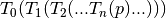 . The semantics are
stack based, that is, first in last applied:
. The semantics are
stack based, that is, first in last applied:
composite_transform <- Transform(T0)
composite_transform$AddTransform(T1)
In the context of registration, if you use a composite transform as the transformation
that is optimized, only the parameters of the last transformation  will
be optimized over.
will
be optimized over.
Additional Resources
- The API for the SimpleITK transformation classes is available in Doxygen format:
- 2D or 3D translation.
- VersorTransform.
- Euler2DTransform and Euler3DTransform.
- Similarity2DTransform and Similarity3DTransform.
- 2D or 3D ScaleTransform.
- ScaleVersor3DTransform.
- ScaleSkewVersor3DTransform.
- 2D or 3D AffineTransform.
- 2D or 3D BSplineTransform.
- 2D or 3D DisplacementFieldTransform.
- Transform.
- To really understand the structure of SimpleITK transforms and how to work with them, we recommend some hands-on interaction using the SimpleITK Jupyter notebooks (Python and R only).
Resampling
Resampling, as the verb implies, is the action of sampling an image, which itself is a sampling of an original continuous signal.
Generally speaking, resampling in SimpleITK involves four components:
- Image - the image we resample, given in coordinate system
 .
. - Resampling grid - a regular grid of points given in coordinate system
 which will be mapped to coordinate system .
 - Transformation
 - maps points from coordinate system
to coordinate system ,
- maps points from coordinate system
to coordinate system ,  .
. - Interpolator - method for obtaining the intensity values at arbitrary points
in coordinate system from the values of the points defined by the Image.
While SimpleITK provides a large number of interpolation methods, the two most commonly used are sitkLinear and sitkNearestNeighbor. The former is used for most interpolation tasks and is a compromise between accuracy and computational efficiency. The later is used to interpolate labeled images representing a segmentation. It is the only interpolation approach which will not introduce new labels into the result.
The SimpleITK interface includes three variants for specifying the resampling grid:
- Use the same grid as defined by the resampled image.
- Provide a second, reference, image which defines the grid.
- Specify the grid using: size, origin, spacing, and direction cosine matrix.
Points that are mapped outside of the resampled image’s spatial extent in physical space are set to a constant pixel value which you provide (default is zero).
Common Errors
It is not uncommon to end up with an empty (all black) image after resampling. This is due to:
- Using wrong settings for the resampling grid (not too common, but does happen).
- Using the inverse of the transformation . This is a relatively
common error, which is readily addressed by invoking the transformation’s
GetInverse method.
Additional Resources
- The API for the SimpleITK ResampleImageFilter class in Doxygen format. The procedural interface for this class supports the three variations for specifying the resampling grid described above.
- To really understand the structure of SimpleITK images and how to work with them we recommend some hands-on interaction using the SimpleITK Jupyter notebooks (Python and R only).